When the Data Refuses to Behave: Building an Agentic Demand Forecasting System

The Problem Nobody Talks About

Ask any supply chain practitioner what keeps them up at night and they will not say “we don’t have enough data.” They will say “we have plenty of data and our forecasts are still wrong.”

This is the honest starting point. Demand forecasting in practice is not a clean regression problem. It is a signal extraction problem embedded in noise - noise from intermittent demand, noise from promotions and events, noise from structural shifts in customer behavior that no historical model can anticipate.

The conventional response has been to throw more sophisticated models at the problem. ARIMA gave way to SARIMA. SARIMA gave way to gradient boosting. Gradient boosting gave way to neural architectures. Each generation of models improved aggregate accuracy while leaving the hard problems - sparse demand, anomalous locations, unknown future events - essentially unsolved.

This project takes a different approach. Instead of asking “what is the best forecasting model?”, we ask “how do we build a system that reasons about forecasts, knows when it is uncertain, and helps a human planner make better decisions?” The answer turns out to involve classical statistics, a modern deep learning architecture, hierarchical reconciliation, and a LLM Agent - not as separate tools, but as an integrated pipeline.

The dataset is the M5 Forecasting Competition dataset from Kaggle(link: https://www.kaggle.com/competitions/m5-forecasting-accuracy/data) - five years of daily Walmart retail sales across 10 stores in three US states. It is the right dataset for this purpose not because it is simple, but because it is genuinely hard. Sixty-eight percent of item-level observations are zero. Some stores behave completely differently from their neighbors. The data has weekly cycles, yearly patterns, event-driven spikes, and government benefit day effects - exactly the complexity we would encounter in pharmaceutical supply chain, fast-moving consumer goods, or industrial parts distribution.

The principles built here transfer directly. Change the dataset, extend the feature set, add domain-specific covariates, and you have a template for any demand-driven supply chain.

The Dataset: M5 Forecasting Competition

The M5 dataset was released by Walmart and the University of Nicosia for the M5 Forecasting Competition in 2020. It is one of the most realistic publicly available retail demand datasets - not sanitised, not aggregated, not simplified.

What It Contains

Five files, each serving a different purpose in the pipeline:

File	Rows	Columns	Contents
sales_train_validation.csv	30,490	1,919	Daily unit sales per item-store, wide format
sales_train_evaluation.csv	30,490	1,947	Same, extended 28 days for final evaluation
sell_prices.csv	6,841,121	4	Weekly sell price per item-store
calendar.csv	1,969	14	Date, day-of-week, events, SNAP flags
sample_submission.csv	60,980	29	Submission format reference

Geography and Hierarchy

Ten stores across three US states, forming a natural four-level hierarchy:

Total (1)
  ├── California (4 stores: CA_1, CA_2, CA_3, CA_4)
  ├── Texas      (3 stores: TX_1, TX_2, TX_3)
  └── Wisconsin  (3 stores: WI_1, WI_2, WI_3)

Each store carries items from three categories - HOBBIES, HOUSEHOLD, FOODS - broken into seven departments. At the bottom of the hierarchy: 3,049 unique items × 10 stores = 30,490 individual time series.

Time Span

1,913 consecutive days of training data from 2011-01-29 to 2016-04-24. The evaluation horizon is 28 days beyond the training window - the same 28-day horizon used throughout this project.

The External Covariates

What makes M5 richer than most retail datasets is the additional context provided per day:

Calendar events - 162 unique event days tagged with a name and type. Event types are Sporting, Cultural, National, and Religious. These are known in advance and can be treated as known future inputs to a forecasting model.

SNAP flags - three binary columns (snap_CA, snap_TX, snap_WI) indicating whether SNAP (Supplemental Nutrition Assistance Program) benefits are distributed on that day in each state. SNAP schedules are determined by state government calendars months in advance - another known future input.

Sell prices - weekly sell price per item-store combination. Prices change over time, vary by store, and are known before the sales period.

Scale

After the wide-to-long transformation:

58,327,370 rows
19 columns per row
10 store partitions on S3
~280 MB total Parquet (compressed)

Why This Dataset Is Representative

The characteristics that make M5 hard are the same characteristics that make real enterprise demand forecasting hard:

• Intermittency at item level: the majority of item-store-day observations are zero. This is standard in pharmaceutical inventory, spare parts, and specialty retail.
• Multi-level hierarchy: procurement, inventory, and financial reporting happen at different aggregation levels and must be consistent.
• Heterogeneous locations: ten stores in the same retail chain behave differently enough that a single model is suboptimal for all of them.
• External covariates with varying importance: prices, events, and benefit days all affect demand, but not equally and not in the way intuition suggests.
• Non-stationarity: all series have trend components requiring explicit differencing or trend modelling.

The dataset does not include everything a real deployment would have - no SKU attributes, no promotions data beyond price, no competitor information, no weather. These are natural extension points for domain-specific implementations.

Phase 1: Getting the Data Right

The M5 dataset arrives as a set of CSV files with a wide format that is immediately impractical for modelling. The central sales file has 30,490 rows - one per item-store combination - and 1,913 columns, one per day. This is a common format in ERP and data warehouse exports, and it is wrong for time series analysis.

The first engineering task is a Bronze -> Silver -> Gold medallion architecture on S3.

Bronze is the raw data landed as Parquet with correct dtypes. The day columns are cast to int16 - maximum Walmart daily item sales fits comfortably in a signed 16-bit integer and this reduces memory footprint by 4x compared to the default float64. This matters because the wide-format sales file is 187MB in Parquet and we need to melt it into 58 million rows.

Silver is where the real transformation happens. The wide-format sales file is melted from 30,490 rows X 1,913 columns to 58,327,370 rows X 19 columns. The sell prices and calendar files are joined in - every sales row now carries its corresponding sell price, day of week, month, year, event flags, and SNAP benefit day indicators.

The memory challenge here is significant. A naive melt of the full dataset requires 27GB of RAM. The solution is a chunked approach - melt one store at a time (3,049 series X 1,913 days = ~5.8M rows), join and write to S3 immediately, then free memory before the next store. Peak memory stays under 2.5GB.

Gold is model-ready output - forecast results and evaluation data - written after each model training run.

Phase 2: Five EDA Questions That Shaped Every Modeling Decision

This is the part most practitioners rush. The five analyses below took longer than any individual model and saved days of misguided experimentation.

2.1 What Does Demand Actually Look Like?

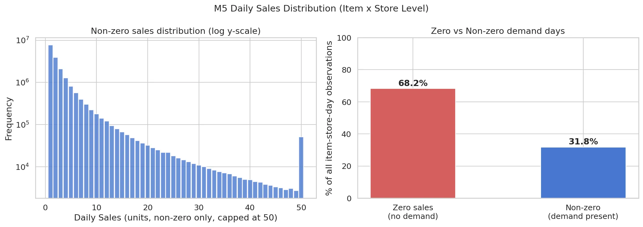
The first and most important finding: 68.2% of all item-store-day observations are zero. Not low - zero. This is not a forecasting problem that a standard ARIMA can solve at the item level. The data is overwhelmingly intermittent.

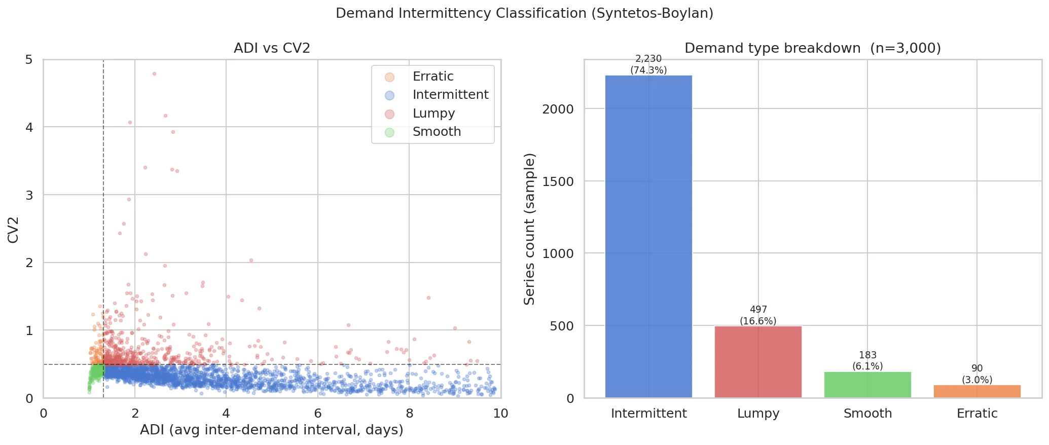
The Syntetos-Boylan classification framework puts a precise label on this. For each series, compute two statistics: ADI (average inter-demand interval, the mean number of days between non-zero observations) and CV-squared (squared coefficient of variation of non-zero demand). The four quadrants - Smooth, Erratic, Intermittent, Lumpy - tell us which model family is appropriate for each series type.

The result: the majority of item-store series fall in the Intermittent and Lumpy quadrants. Standard models will systematically overforecast because they cannot represent the structural zeros.

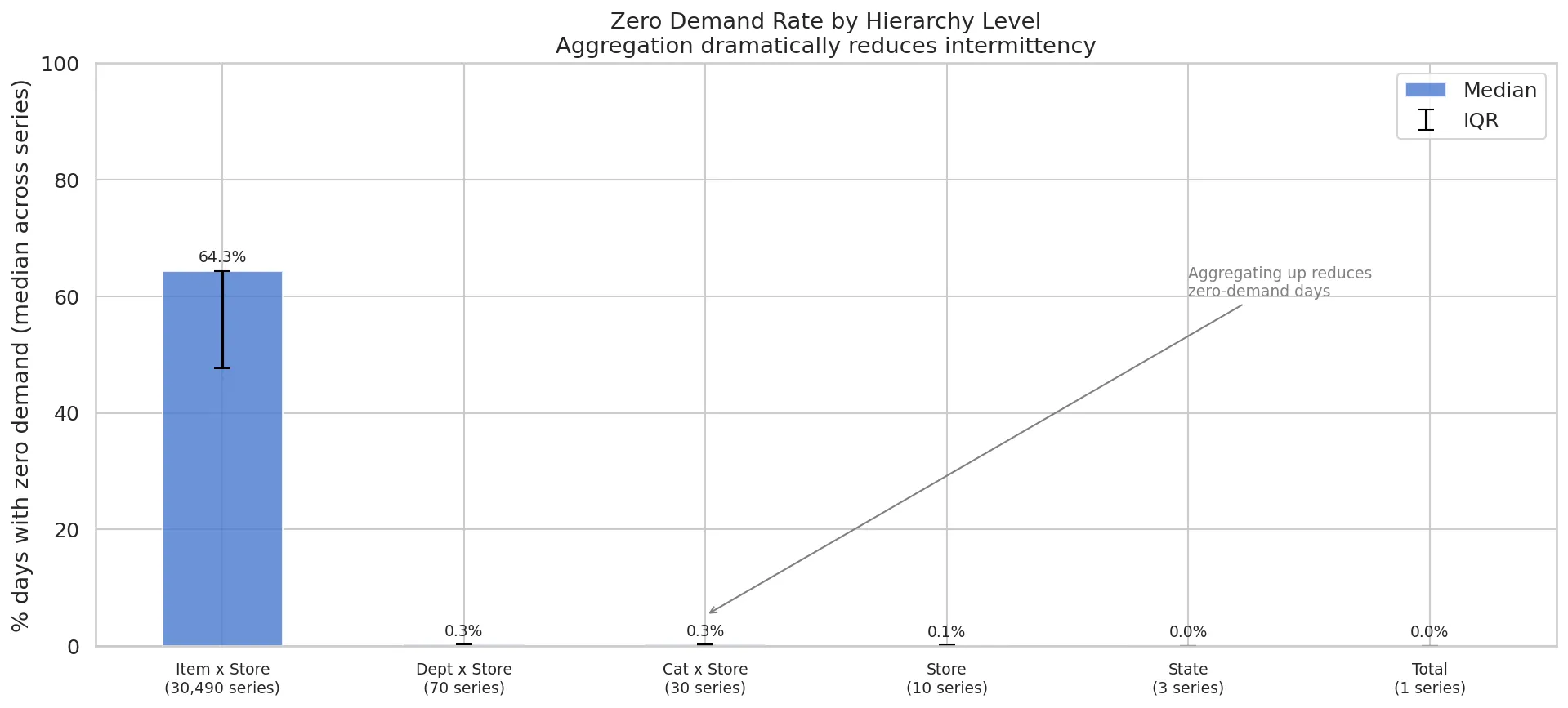
This finding drove a fundamental architectural decision: do not attempt to forecast at item-store level with classical models. Instead, aggregate up the hierarchy until the signal is clean, forecast there, and disaggregate.

2.2 How Does Aggregation Change the Signal?

Level	Series Count	Median Zero%	Median CV
Item X Store	30,490	64.3%	1.84
Dept X Store	70	0.3%	0.32
Cat X Store	30	0.3%	0.29
Store	10	0.1%	0.23
State	3	0.0%	0.22
Total	1	0.0%	0.21

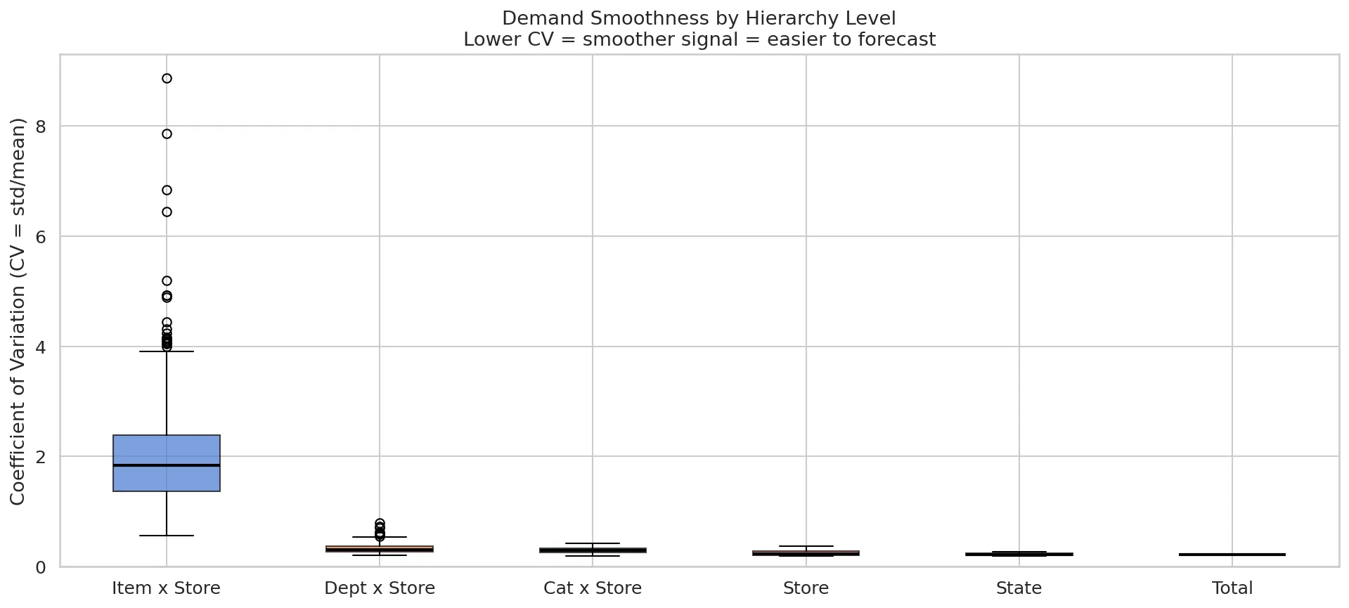
The cliff between item-store and department-store level is dramatic. Zero rate drops from 64% to 0.3% in a single aggregation step. CV drops from 1.84 to 0.32. The signal completely transforms.

This table determined the model assignment strategy:

• SARIMA operates at store level (CV 0.23, zero% 0.1%) - smooth enough for classical time series
• Prophet operates at store level for direct comparison
• TFT operates at store level with quantile loss - handles the residual intermittency in the 28-day horizon

2.3 Is There a Seasonal Structure Worth Modelling?

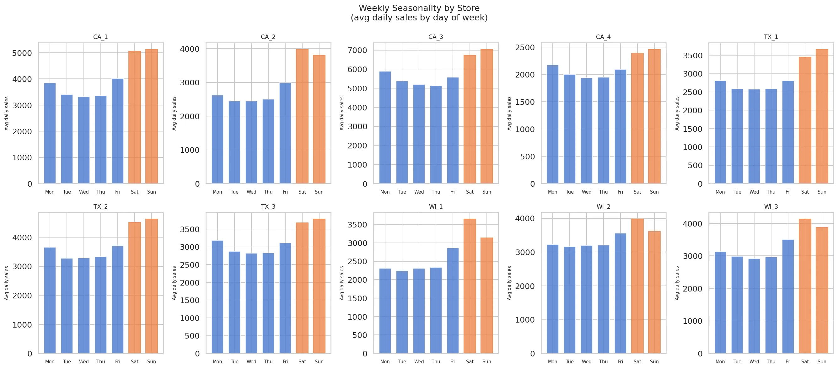
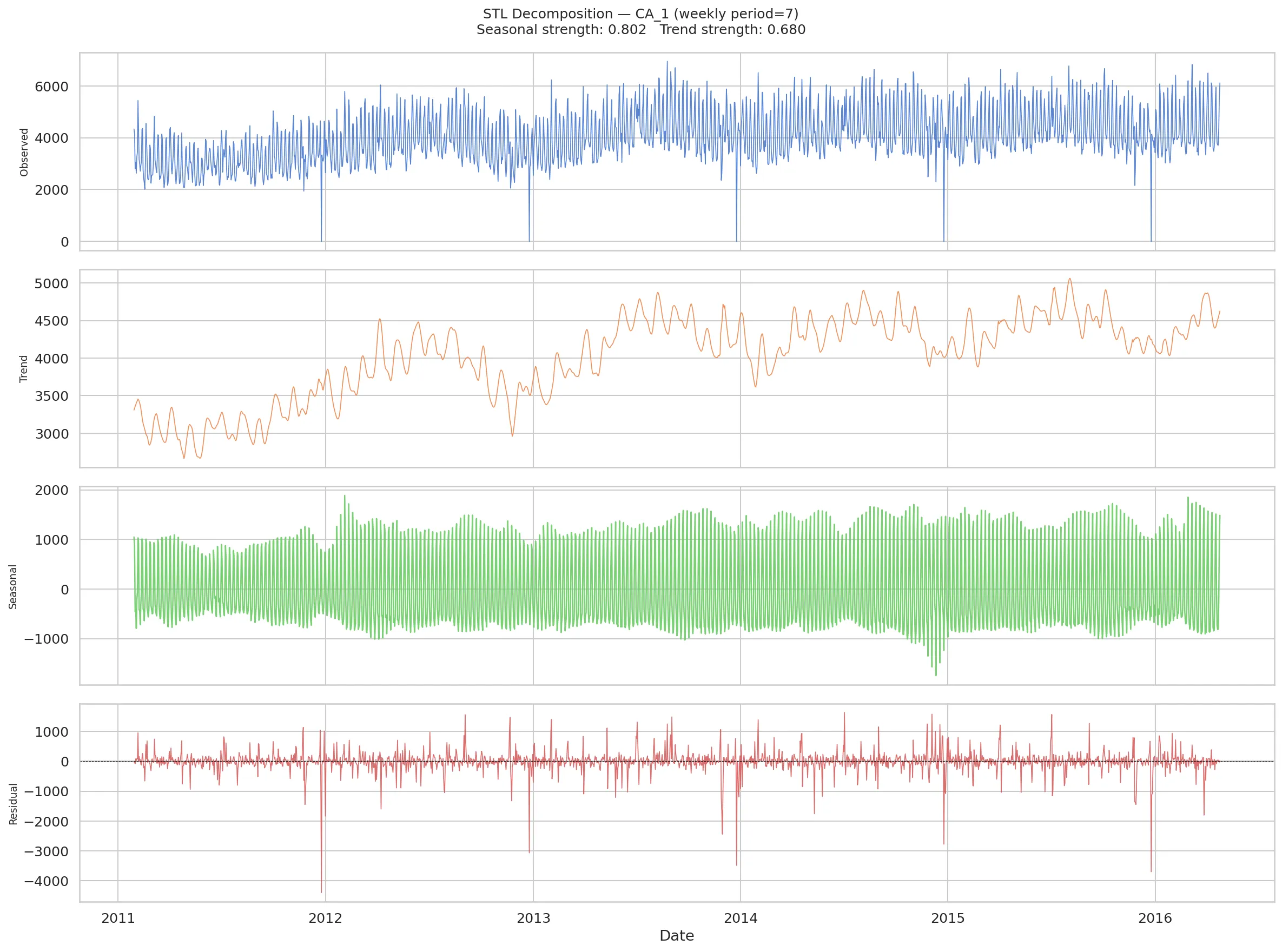
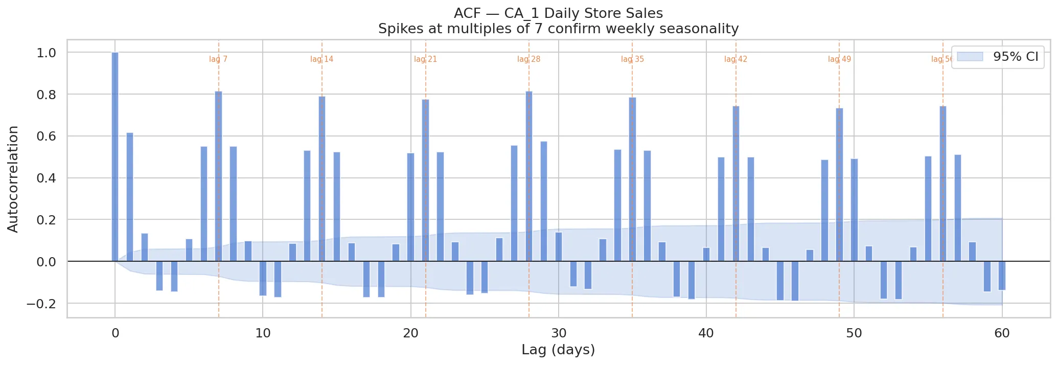
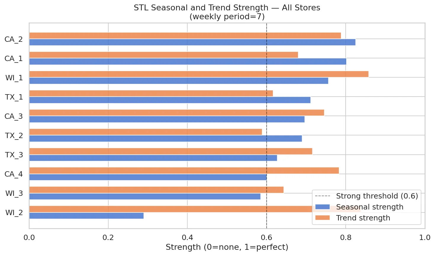
STL decomposition (Seasonal and Trend decomposition using Loess) at store level reveals seasonal strength values of 0.6-0.8 for most stores, confirming strong weekly seasonality. The ACF plot makes this visually explicit - significant spikes at lags 7, 14, 21, 28, 35, 42, 49, and 56. Every multiple of 7 is significant.

This confirmed SARIMA’s seasonal order as (1,1,1,7) and Prophet’s weekly_seasonality=True without any guesswork.

One important anomaly: WI_2 has seasonal strength of only 0.29, while every other store is above 0.6. This single number predicted, before a single model was trained, that SARIMA would perform poorly on WI_2. It did - RMSSE of 1.93, worse than the naive baseline.

2.4 Do External Signals Actually Move Demand?

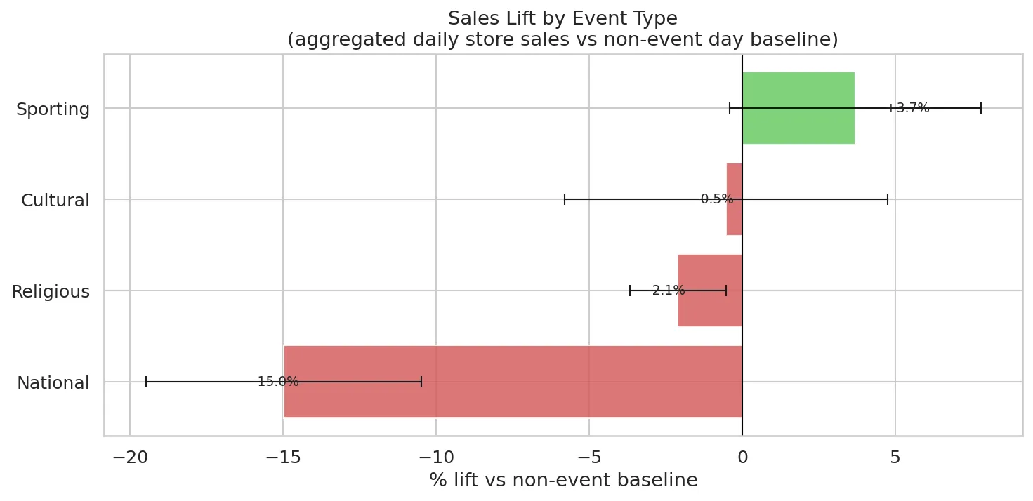
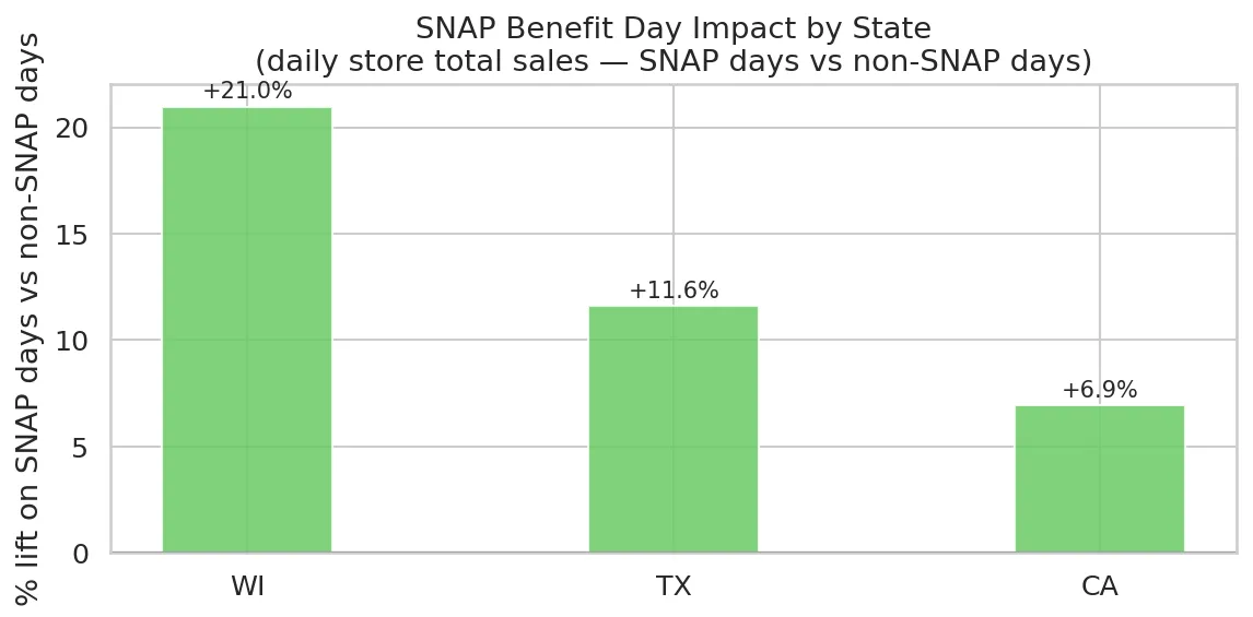
Three external signals in the M5 data: sell price, calendar events, and SNAP benefit day flags. Each needed empirical validation before including it as a TFT covariate.

Calendar events: National holidays drive a -15% demand drop - stores close or reduce hours, and shopping is deferred. Sporting events drive a +3.7% lift - people stock up before games. This is not symmetrical, and a model that treats all events the same will be consistently wrong.

SNAP benefit days: The government food assistance programme releases benefits on specific days of the month. The lift is striking - WI +21%, TX +12%, CA +7%. Wisconsin’s high SNAP participation rate relative to its store count explains why WI_2 is anomalous in multiple ways. These are real government programme effects that can be looked up in advance and encoded as known future inputs to TFT.

Price: A +65.8% sales difference between lowest and highest price quintiles sounds like strong elasticity. It is not - it is a confound. Higher-priced items tend to be premium products with higher inherent volume. True within-item price elasticity is much weaker. Sell price is still included as a TFT covariate but interpreted carefully.

2.5 What Differencing Do the Series Need?

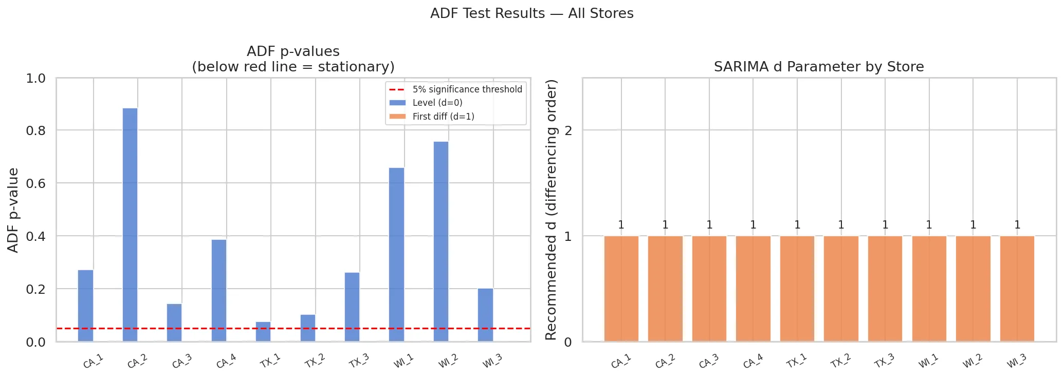
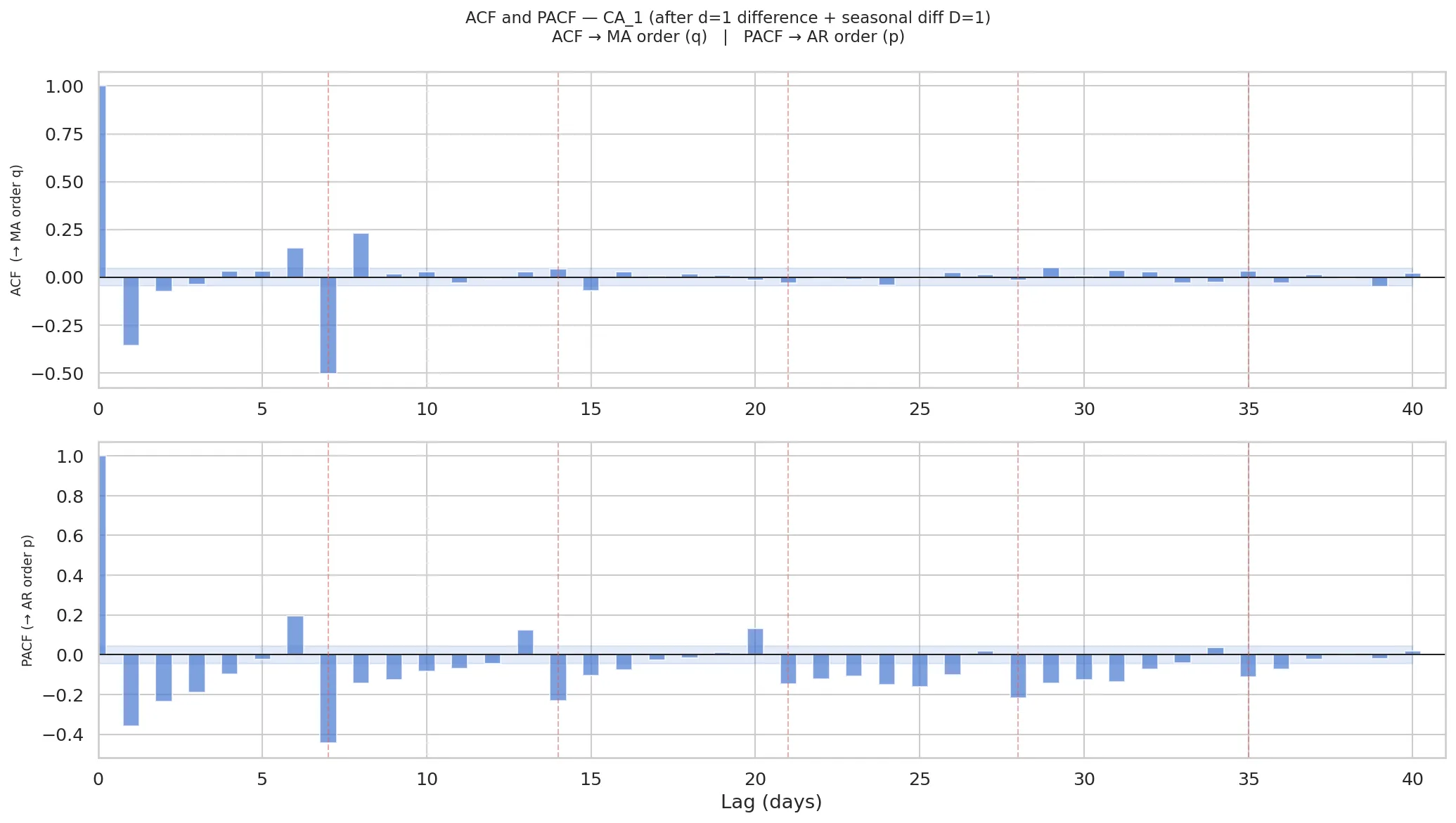
Augmented Dickey-Fuller tests on all 10 store series. Result: all 10 are non-stationary at level (unit root present) and stationary after first difference. ADF p-values after first differencing are 0.0000 across the board.

This means every store series is I(1) - integrated of order 1. SARIMA needs d=1. The ACF and PACF plots after first differencing show spikes at lag 7 in both, confirming P=1, Q=1 seasonal terms.

Final confirmed SARIMA order from first principles: SARIMA(1,1,1)(1,1,1,7).

Phase 3: Three Models, One Benchmark

SARIMA - The Classical Baseline

SARIMA fits one model per store series. The mathematics are well understood - maximum likelihood estimation of AR, MA, and seasonal components after differencing to achieve stationarity. It has no ability to use external covariates, cannot learn cross-series patterns, and assumes the seasonal structure is fixed. Its strength is interpretability and reliability on well-behaved series.

Results:

Store	RMSSE	vs Naive
CA_1	0.4145	-58%
CA_2	0.5426	-46%
CA_3	0.4479	-55%
CA_4	0.4914	-51%
TX_1	0.3340	-67%
TX_2	0.4756	-52%
TX_3	0.5240	-48%
WI_1	0.4738	-53%
WI_2	1.9301	-97% worse
WI_3	0.6291	-37%
Mean	0.6263	-37%

WI_2 at 1.9301 is the immediate signal. The model has learned a seasonal structure that does not match this store’s actual demand pattern. It is predicting weekly cycles that do not materialise.

Prophet: Trend-Adaptive Decomposition

Prophet models demand as a sum of trend (with automatic changepoint detection), weekly seasonality, yearly seasonality, and holiday effects. It is substantially more flexible than SARIMA in handling trend shifts and does not require specifying differencing orders.

Three design choices driven by EDA:

1. Multiplicative seasonality: seasonal swings should scale with trend level, not remain additive
2. Holiday windows: national holidays get lower_window=-1, upper_window=1 to capture the day-before shopping surge and day-after recovery
3. Log1p transform: stabilises variance across stores with very different volume levels

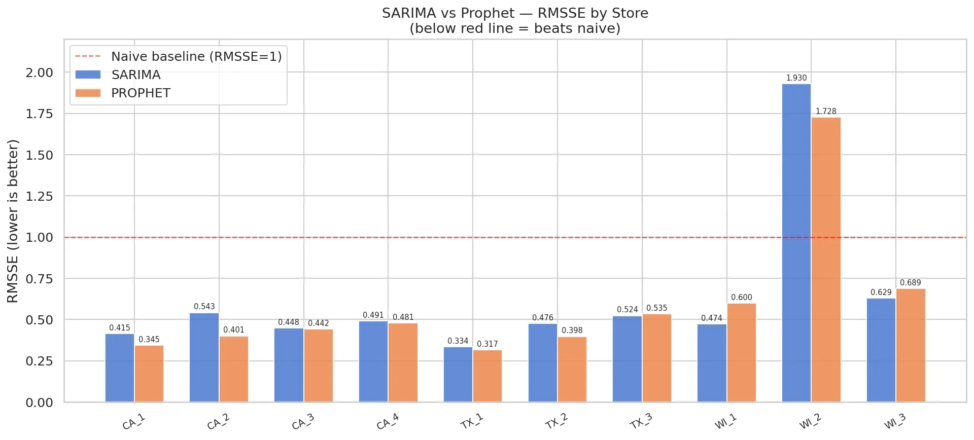
Results:

Store	Prophet	SARIMA	Winner
CA_1	0.3454	0.4145	Prophet +0.069
CA_2	0.4010	0.5426	Prophet +0.142
CA_3	0.4419	0.4479	Prophet +0.006
CA_4	0.4807	0.4914	Prophet +0.011
TX_1	0.3175	0.3340	Prophet +0.017
TX_2	0.3982	0.4756	Prophet +0.077
TX_3	0.5352	0.5240	SARIMA +0.011
WI_1	0.6002	0.4738	SARIMA +0.126
WI_2	1.7277	1.9301	Prophet +0.202
WI_3	0.6887	0.6291	SARIMA +0.060
Mean	0.5937	0.6263	Prophet

Prophet wins 7/10 stores and reduces mean RMSSE from 0.6263 to 0.5937. WI_2 improves meaningfully from 1.93 to 1.73 - still above the naive baseline, but the direction is right.

The Wisconsin stores reveal something interesting. WI_2 improves with Prophet, but WI_1 and WI_3 get worse. Three stores in the same state, three different model preferences. This heterogeneity is the core argument for best-model-per-store routing rather than a single model for all locations.

Phase 4: Temporal Fusion Transformer(TFT)

Why TFT for This Problem?

The Temporal Fusion Transformer (Lim et al., 2021) was designed for exactly this type of problem. Its architecture handles multiple input types simultaneously:

• Static metadata: store identity, state identity (things that do not change)
• Known future inputs: day of week, month, events, SNAP flags, sell price (things we know in advance)
• Unknown past inputs: historical sales (things we only know historically)

The multi-head attention mechanism learns which time steps in the encoder window matter most for each forecast horizon step. For a store with strong weekly seasonality, it learns to attend to the same day of the prior week. For a store with irregular demand, it learns to attend to longer-range patterns.

Critically, TFT produces quantile forecasts natively. Instead of predicting one number, it simultaneously predicts the 10th, 50th, and 90th percentile. This is not a post-processing step - it is trained end-to-end with quantile loss. For a supply chain planner, the 10th percentile is a pessimistic scenario (plan minimum order), the 90th percentile is an optimistic scenario (plan safety stock), and the 50th is the point forecast.

Architecture Configuration

Derived directly from EDA findings:

encoder_length    = 90 days    (covers 13 weekly cycles - confirmed by ACF)
prediction_length = 28 days    (matches evaluation horizon)
hidden_size       = 64         (conservative - avoids overfitting on ~1,885 training days)
lstm_layers       = 2
attention_heads   = 4
dropout           = 0.1
quantiles         = [0.1, 0.5, 0.9]
loss              = QuantileLoss

Known future inputs: wday, month, is_event, is_snap, sell_price
Static categoricals: store_id, state_id

Training used early stopping with patience=5 on validation loss, GPU acceleration on an NVIDIA RTX 3050 Ti, and MLflow experiment tracking.

Results

Store	TFT	Prophet	SARIMA	Best
CA_1	0.2508	0.3454	0.4145	TFT
CA_2	0.4505	0.4010	0.5426	Prophet
CA_3	0.2915	0.4419	0.4479	TFT
CA_4	0.4819	0.4807	0.4914	Prophet (marginal)
TX_1	0.2832	0.3175	0.3340	TFT
TX_2	0.3040	0.3982	0.4756	TFT
TX_3	0.5659	0.5352	0.5240	SARIMA
WI_1	0.6102	0.6002	0.4738	SARIMA
WI_2	1.1662	1.7277	1.9301	TFT
WI_3	0.5354	0.6887	0.6291	TFT
Mean	0.4940	0.5937	0.6263	TFT
WRMSSE	~0.49	0.5867	0.6219	TFT

TFT achieves mean RMSSE of 0.4940 - below the stretch goal of 0.50. It beats Prophet on 6/10 stores and beats SARIMA on 7/10.

The WI_2 story is the most instructive. SARIMA 1.93 -> Prophet 1.73 -> TFT 1.17. Three models, each better than the previous, none fully solving it. WI_2 is still above the naive baseline. This is not a failure of modelling - it is an honest signal that this location’s demand has structural unpredictability that historical data cannot resolve. The right response is not more model complexity; it is flagging this location for human review and building a system that does that automatically.

The two stores where classical models beat TFT - TX_3 and WI_1 - have very regular, stationary demand. SARIMA’s simplicity is an advantage there. The bias-variance tradeoff is real: TFT’s additional complexity introduces variance that hurts on easy series.

Phase 5: Serving - Best-Model-Per-Store Routing

The serving layer implements a routing table that selects the best model per store based on validation RMSSE. This is a more honest approach than deploying a single model universally and pretending it is optimal everywhere.

ROUTING_TABLE = {
    "CA_1": ("tft",     0.2508),   # TFT strong win
    "CA_2": ("prophet", 0.4010),   # Prophet wins
    "CA_3": ("tft",     0.2915),   # TFT strong win
    "CA_4": ("prophet", 0.4807),   # Prophet marginal win
    "TX_1": ("tft",     0.2832),   # TFT wins
    "TX_2": ("tft",     0.3040),   # TFT wins
    "TX_3": ("sarima",  0.5240),   # SARIMA wins on regular demand
    "WI_1": ("sarima",  0.4738),   # SARIMA wins on regular demand
    "WI_2": ("tft",     1.1662),   # TFT best available (flag for review)
    "WI_3": ("tft",     0.5354),   # TFT wins
}

The FastAPI service exposes five endpoints:

• GET /forecast/{store_id} - best model forecast (uses routing table)
• GET /forecast/{store_id}?model=tft - force a specific model
• GET /forecast/{store_id}/compare - all three models side by side
• POST /forecast/batch - multiple stores in one call
• GET /routing - the full routing table with rationale

The compare endpoint is particularly useful for building planner intuition - seeing when TFT and Prophet disagree strongly is itself a signal of forecast uncertainty.

Phase 6: SupplyMind - The Agentic Layer

This is where the project becomes something qualitatively different from a forecasting pipeline.

The Problem With Point Forecasts Alone

A number without context is not a decision. A planner looking at “CA_1 forecast: 12,400 units/day for the next 28 days” needs to know: is that high or low relative to history? What is the uncertainty? Are there specific days that are risky? What should I actually do?

These questions require reasoning, not computation. The SupplyMind agent uses Claude Sonnet 4.5 (Anthropic’s language model) in a multi-turn conversational mode to reason over forecast outputs and generate actionable inventory recommendations.

System Design

The agent maintains a session per store. When a session is created:

1. The forecast is loaded from S3 Gold
2. Statistical signals are computed programmatically (spike detection, uncertainty flags, trend direction)
3. All of this context is injected into the first message to the model
4. The model generates an initial analysis
5. The planner can ask any follow-up questions in natural language

The system prompt encodes supply chain domain knowledge: EOQ logic, safety stock calculation, the FINDING -> DRIVER -> ACTION -> RISK communication structure, and explicit instructions to flag situations requiring human escalation.

What the Agent Actually Says

Here is an excerpt from the initial analysis for TX_1 (lightly edited for space):

FINDING: Stable, high-volume demand with moderate weekly cyclicality and slight downward drift.

RISK: Systematic Overforecasting. Model overforecasts by 5-20% on 60% of days, particularly weekends. This could be an Easter timing effect - Easter 2016 was March 27, earlier than in the training period.

ACTION 1: Reduce safety stock by 8-10% for Weeks 2-4. Downward trend (-3.8%) plus systematic overforecasting suggests lower stockout risk than the model implies. Implement from April 1 after the first week validates the pattern.

ESCALATE: Investigate systematic forecast bias. Questions for human expert: Was there a promotional calendar shift in 2016? Did a competitor open nearby in Q1?

This is not a template. The model noticed the Easter timing effect independently by examining the specific dates and recognising the deviation from the weekly pattern.

Multi-Turn Reasoning

When the planner mentions a local festival in week 3, the agent:

1. Immediately flags that TFT does not know about this event (it is outside the training distribution)
2. Builds three demand scenarios - Moderate (+20-30%), Major (+40-60%), Mega (+75-100%) - with specific unit numbers per scenario
3. Cancels its own previous recommendation (“Reduce safety stock - now INVALID for Week 3”)
4. Provides a revised safety stock calendar with dynamic targets by week
5. Lists the specific questions the planner needs to answer before the recommendation can be finalised

The willingness to revise its own prior recommendation based on new information is the behaviour that distinguishes a useful agent from a static report generator.

Phase 7: MinT Hierarchical Reconciliation

A supply chain operates at multiple levels simultaneously. Procurement happens at category level, inventory planning happens at store level, financial reporting happens at state and total level. If the forecasts at each level are produced independently, they will not sum correctly - and a planner reconciling different reports will see different numbers for the same business.

MinT (Minimum Trace reconciliation, Wickramasuriya et al. 2019) solves this by finding the optimal linear correction to all hierarchy levels simultaneously, minimising total forecast error while guaranteeing that store forecasts sum exactly to state forecasts, which sum exactly to the total forecast.

The key equation: $ỹ_{bottom} = (S’W^{-1}S)^{-1} S’W^{-1} × (S × ŷ_{bottom})$

Where S is the summing matrix encoding the hierarchy structure, W is the covariance matrix of base forecast errors estimated with Ledoit-Wolf shrinkage, and ỹ is the reconciled forecast.

The coherence verification after reconciliation confirmed all constraints satisfied - store forecasts sum to state, state forecasts sum to total - to within floating point tolerance.

In this project, since all models were trained at store level only (no independent state or total models), the reconciliation adjustment is zero by construction. The value of having this layer in the architecture is that when you extend the system with top-down models - as you would in a real enterprise deployment where category managers produce their own demand plans - the MinT layer will automatically reconcile the conflict between bottom-up store forecasts and top-down category plans.

What the Numbers Say - and What They Don’t

The Scorecard

Model	Mean RMSSE	WRMSSE	Stores Won
Naive baseline	1.0000	1.0000	-
SARIMA	0.6263	0.6219	3/10
Prophet	0.5937	0.5867	4/10
TFT	0.4940	~0.49	6/10
Best-per-store ensemble	0.4378	-	10/10

The ensemble - simply routing each store to its best model - achieves 0.4378, the best result. This is not a sophisticated method. It is the honest acknowledgement that no single model dominates everywhere and that selecting the right tool per context is itself a modelling decision.

What Remains Hard

WI_2 at RMSSE 1.17 after TFT. Better than SARIMA (1.93) and Prophet (1.73), but still worse than a naive random walk. Three of the best forecasting approaches in the literature, none able to beat naive on this single location.

This is not a failure. It is information. It tells the supply planner: this location requires a fundamentally different approach - either better data (more granular external signals, local event calendars, competitor information), more training history, or an acceptance that demand here is structurally stochastic at this forecasting horizon.

The agent is designed to surface exactly this. WI_2 gets a warning in every analysis it generates: RMSSE > 1.0, this forecast is less accurate than a naive baseline, treat with caution, escalate to human review. That is honest and useful in a way that a dashboard showing just the forecast number is not.

Extending This to Real Enterprise Problems

This project was built on Walmart retail data, but the architecture is directly applicable to more complex domains. A few extensions worth considering:

Pharmaceutical supply chain: Replace sell prices with tender prices and contract values. Replace SNAP flags with quarter-end budget flush effects. Replace event types with therapy area launch cycles and genericisation events. The intermittency problem is worse in pharma - many specialty products sell zero units in most markets in most weeks. The hierarchy is richer - SKU -> presentation -> brand -> therapy area -> market -> global.

Industrial parts distribution: The demand signal is driven by maintenance cycles, equipment age distributions, and failure rates - none of which appear in historical sales data directly. Adding equipment fleet data as a known future covariate to TFT is a meaningful extension.

Multi-echelon inventory: This project forecasts demand at the point of sale. In practice, a manufacturer needs to forecast demand at the distribution centre level, accounting for retailer ordering patterns which are themselves driven by their own forecasting decisions. The hierarchy reconciliation layer is the right place to model these cross-echelon constraints.

Real-time retraining: This implementation uses static models trained once and served from pre-computed forecasts. A production system would trigger retraining on a rolling basis as new sales data arrives, using the same MLflow experiment tracking structure to compare new models against incumbents before promoting them.

Lessons Learned

EDA is not a formality. The decision to use TFT with quantile loss, to route SARIMA to store level only, and to encode SNAP flags as known future inputs - every one of these came directly from the five EDA analyses. Skipping EDA and jumping to model training would have produced a less accurate system and, more importantly, a system whose failure modes were invisible.

The anomalous location is the most important signal. WI_2 was flagged in EDA 3 (seasonal strength 0.29), confirmed broken in Phase 3 (SARIMA RMSSE 1.93), and partially recovered by TFT (1.17) but not solved. Following one anomalous location through the entire pipeline taught more about the limits of historical forecasting than the nine well-behaved stores combined.

Uncertainty quantification is not optional. Prophet and TFT both produce prediction intervals. SARIMA produces them too. A system that reports only point forecasts is discarding valuable information - the width of the interval tells the planner how much safety stock is justified. A 28-day forecast with a 3,000-unit prediction interval band is a fundamentally different planning input than one with a 300-unit band, even if both have the same point forecast.

The agent layer changes the conversation. When the store manager mentioned a local festival and the agent revised its own safety stock recommendation, cancelled a prior action item, and asked specific clarifying questions - that is a different quality of decision support than any static report or dashboard can provide. The value is not in the AI doing the planning; it is in the AI making the human planner’s reasoning more rigorous and the relevant information more visible.

Best-model-per-store is better than one-model-everywhere. This seems obvious but it contradicts the standard practice of selecting a single modelling approach for an entire dataset. TX_3 and WI_1 are better served by SARIMA than by TFT. Acknowledging this and routing accordingly is intellectually honest and operationally superior.

Technical Stack Summary

Component	Technology	Why
Data lake	AWS S3 + Athena	Serverless query, near-zero cost at M5 scale
Data processing	pandas, pyarrow	Chunked processing for 58M row melt
Classical forecasting	statsmodels SARIMAX	Transparent, mathematically grounded
Decomposition forecasting	Prophet	Handles trend changepoints, holiday effects
Deep learning	PyTorch + pytorch-forecasting TFT	Native quantile output, handles covariates
Experiment tracking	MLflow (self-hosted)	Portable, no vendor lock-in
Serving	FastAPI	Async, production-grade, minimal overhead
Agentic reasoning	Claude API (Anthropic)	Multi-turn conversation, supply chain reasoning
Reconciliation	MinT-Shrink (numpy)	Optimal hierarchical coherence
Deployment	AWS EKS (eksctl)	Kubernetes for production serving
Package management	uv	Fast, reproducible Python environments

Conclusion

The question this project started with was not “what model should I use for demand forecasting?” It was “how do I build a system that forecasts well, knows when it is uncertain, and helps a human planner make better decisions?”

The answer required three things to work together: models that capture different aspects of the demand signal, a reconciliation layer that makes forecasts coherent across planning levels, and an agent that reasons about forecast outputs in the context of operational decisions.

No single model solved WI_2. No amount of feature engineering made intermittent item-level demand tractable for classical approaches. But the combination - best-model routing, quantile uncertainty, human-in-the-loop escalation via the agent - produced a system that is honest about what it knows and useful about what to do with it.

That combination is, ultimately, what the “agentic approach” to demand forecasting means in practice. Not an autonomous system that makes inventory decisions. A system that does the quantitative heavy lifting, surfaces what matters, and makes the human decision-maker more effective.

Glossary

ACF (Autocorrelation Function): A statistical measure of the correlation between a time series and lagged versions of itself. Spikes at specific lags reveal periodic patterns. In this project, ACF spikes at lags 7, 14, 21 confirmed weekly seasonality and informed the SARIMA seasonal order.

ADI (Average Inter-Demand Interval): The average number of days between non-zero demand observations for an item. High ADI indicates intermittent demand. Used in the Syntetos-Boylan classification framework alongside CV² to categorise series into Smooth, Erratic, Intermittent, or Lumpy.

ADF (Augmented Dickey-Fuller Test): A statistical hypothesis test for the presence of a unit root in a time series. A unit root implies non-stationarity - the series has a trend that does not revert to a fixed mean. If the ADF p-value is above 0.05, the series is non-stationary and requires differencing before ARIMA-family models can be applied.

AIC (Akaike Information Criterion): A measure of statistical model quality that penalises complexity. Lower AIC indicates a better trade-off between model fit and number of parameters. Used to compare fitted SARIMA models.

Agentic AI: An AI system that takes actions, reasons over information, and produces outputs beyond simple question-answering. In this project, the SupplyMind agent loads forecast data, computes statistical signals, generates an initial analysis, and engages in multi-turn reasoning to answer follow-up questions and revise recommendations.

AR (Autoregressive): A model component where the current value of a series depends linearly on its own past values. The order p in ARIMA(p,d,q) specifies how many past observations are included.

ARIMA: Autoregressive Integrated Moving Average. A family of time series forecasting models combining autoregression (AR), differencing (I) to achieve stationarity, and moving average (MA) components. SARIMA extends ARIMA with seasonal terms.

Bronze / Silver / Gold: A data lake architecture pattern (also called the medallion architecture) where raw data lands in Bronze with minimal transformation, Silver applies cleaning and joins, and Gold contains model-ready and analysis-ready outputs. Borrowed from data engineering best practice and applied here to the S3 data lake.

CV² (Squared Coefficient of Variation): The square of the ratio of standard deviation to mean, computed on non-zero demand observations only. Low CV² means demand quantity is consistent when it occurs (smooth or intermittent). High CV² means demand quantity is erratic when it occurs.

EOQ (Economic Order Quantity): A classic inventory management formula that determines the optimal order quantity minimising total holding and ordering costs. Assumes constant demand - in practice, used as a baseline adjusted by forecast uncertainty.

EKS (Elastic Kubernetes Service): Amazon Web Services’ managed Kubernetes service. Used here for the final production deployment of the FastAPI inference service, providing container orchestration, auto-scaling, and high availability.

HiTL (Human-in-the-Loop): A system design principle where automated decisions are reviewed and approved by a human before being acted upon. In this project, the agent generates recommendations but does not trigger inventory actions directly - a planner reviews and approves.

I(d) / Integrated of Order d: A time series is I(d) if it becomes stationary after d differences. All 10 store series in this project are I(1) - one round of first-differencing removes the unit root and achieves stationarity.

Intermittent Demand: A demand pattern characterised by many zero observations interspersed with non-zero demand. Common in specialty retail, pharmaceutical inventory, spare parts, and any product with low average demand relative to the forecasting period.

LSTM (Long Short-Term Memory): A type of recurrent neural network architecture designed to capture long-range dependencies in sequential data. TFT uses LSTM layers as part of its encoder-decoder structure.

MA (Moving Average): A model component where the current value depends on past forecast errors (residuals). The order q in ARIMA(p,d,q) specifies how many past errors are included. Not to be confused with a simple moving average used in technical analysis.

MAPE (Mean Absolute Percentage Error): A forecast accuracy metric expressing average error as a percentage of actual values. Undefined when actuals are zero, which makes it poorly suited for intermittent demand series.

MinT (Minimum Trace Reconciliation): A method for reconciling forecasts across a hierarchy so that lower-level forecasts sum exactly to upper-level forecasts. Finds the optimal linear correction minimising the trace of the forecast error covariance matrix. Named for the mathematical property it optimises.

MLflow: An open-source platform for managing the machine learning lifecycle, including experiment tracking, model versioning, and artifact storage. Used here to log every model training run with parameters, metrics, and forecast outputs.

PACF (Partial Autocorrelation Function): Similar to ACF, but measures the correlation between a time series and a lagged version after removing the effect of intermediate lags. Spikes in PACF indicate the appropriate AR order for an ARIMA model.

Prophet: A forecasting library developed by Meta (Facebook) that models time series as a sum of trend, seasonality, and holiday components. Designed to handle series with multiple seasonalities, trend changepoints, and irregular holidays without manual parameter specification.

Quantile Forecasting: Predicting specific percentiles of the future demand distribution rather than a single point estimate. A model that predicts the 10th, 50th, and 90th percentile gives the planner a pessimistic scenario, a central estimate, and an optimistic scenario simultaneously - directly informing safety stock calculations.

RMSSE (Root Mean Squared Scaled Error): The primary per-series accuracy metric used in the M5 competition. Computed as the square root of the ratio of mean squared forecast error to the mean squared naive (random walk) forecast error on the training data. RMSSE < 1 means the model beats the naive baseline; RMSSE = 1 means it equals it; RMSSE > 1 means naive is better.

Safety Stock: Inventory held above the expected demand level to buffer against forecast uncertainty and supply variability. Higher forecast uncertainty justifies higher safety stock. Calculated as Z × σ_demand × √(lead_time), where Z is the service level factor and σ_demand is the standard deviation of demand.

SARIMA (Seasonal ARIMA): An extension of ARIMA that explicitly models seasonal patterns. The notation SARIMA(p,d,q)(P,D,Q,s) adds seasonal AR (P), seasonal differencing (D), seasonal MA (Q), and seasonality period (s) terms to the standard ARIMA components. In this project: SARIMA(1,1,1)(1,1,1,7) for weekly seasonality.

SNAP (Supplemental Nutrition Assistance Program): A US federal programme providing food purchase assistance to low-income households. Benefits are distributed on specific days of the month that vary by state. These days are known in advance and produce measurable demand spikes at food retailers.

STL (Seasonal and Trend Decomposition using Loess): A decomposition method that separates a time series into trend, seasonal, and residual components using locally weighted regression (Loess). Robust to outliers. Used in this project to measure seasonal and trend strength and to confirm the weekly seasonal structure.

Summing Matrix (S): In hierarchical forecasting, a matrix that encodes the aggregation structure of a hierarchy. Multiplying the bottom-level forecasts by S produces forecasts at all levels simultaneously. Used in the MinT reconciliation formula.

TFT (Temporal Fusion Transformer): A deep learning architecture for multi-horizon time series forecasting, introduced by Lim et al. (2021). Combines LSTM sequence encoding with multi-head attention to learn which historical time steps matter most for each forecast horizon, while handling static metadata, known future covariates, and past observed variables in a unified architecture.

WRMSSE (Weighted Root Mean Squared Scaled Error): The official M5 competition metric. A weighted average of per-series RMSSE scores where weights are proportional to each series’ contribution to total training sales. Higher-volume series matter more.

Appendix: A Conversation from Chatbot

# DEMAND ANALYSIS: TX_1 (2016-03-25 to 2016-04-21)

## 1. OVERALL DEMAND OUTLOOK

**FINDING:** Stable, high-volume demand with moderate weekly cyclicality and slight downward drift.

- **Volume:** 12,436 units/day average (~87K units/week) - this is a high-volume store
- **Pattern:** Weekly peaks on Saturdays (Mar 27, Apr 3, Apr 9, Apr 16 show elevated forecasts 13.5K-14.5K units)
- **Trend:** Modest decline of 3.8% from week 1 to week 4 (14.5K peak -> 12.3K by end)
- **Model confidence:** Strong. RMSSE of 0.28 means TFT is 72% more accurate than naive baseline. Actual performance validates this - most days within 80% prediction intervals.

**No major demand shocks expected.** This is a predictable, mature demand pattern.

---

## 2. KEY RISKS & ANOMALIES

### **RISK 1: Forecast-Actual Mismatch Pattern (Systematic Overforecasting)**
- **Days 1-3 (Mar 25-27):** Forecast overshot actuals by 10-13% (predicted 12.4K-14.5K, actual 11.3K-12.8K)
- **Days 9-10 (Apr 2-3):** Forecast 13.6K-14.4K, actual only 11.4K-11.7K (19-23% miss)
- **Impact:** Risk of excess inventory buildup if this pattern continues

**DRIVER:** Possible Easter timing effect (Easter 2016 = March 27) or promotional calendar shift not fully captured by TFT. Model may be anchoring to prior year patterns that don't align.

### **RISK 2: Forecast Volatility vs. Actual Stability**
- **Forecast range:** 10.5K-14.5K (38% swing)
- **Actual range:** 10.3K-13.7K (33% swing, but tighter clustering around 11.5K-12.5K)
- **Issue:** Model predicts more volatility than materializes, particularly overestimating Saturday peaks

**DRIVER:** TFT may be overfitting to historical weekend spikes that are moderating in 2016.

### **LOW RISK: Uncertainty Quantification**
- No days with PI ratio >2.0x (prediction intervals are appropriately sized)
- 80% PIs consistently span ~3K units, reasonable for this volume
- No extreme outlier days flagged

---

## 3. TOP INVENTORY ACTIONS

### **ACTION 1: Reduce Safety Stock by 8-10% for Weeks 2-4**
- **Rationale:** Downward trend (-3.8%) + systematic overforecasting = lower risk of stockouts than model suggests
- **Specific:** If current safety stock targets ~2,500 units (2 days of mean demand), reduce to ~2,250 units
- **Timing:** Implement starting April 1 (after initial week validates pattern)
- **Risk mitigation:** Monitor daily sell-through rates. If actuals exceed forecast 3+ consecutive days, revert to standard safety stock.

### **ACTION 2: Dampen Saturday Replenishment by 12-15%**
- **Rationale:** Forecasted Saturday peaks (14K-14.5K) consistently overshoot actuals by 1.5K-2K units
- **Specific:** For Saturdays Apr 9, 16, 23, order to 13K target instead of 14K+
- **Expected benefit:** Avoid 4K-6K units of excess inventory across 3 Saturdays
- **Validation:** Compare Apr 9 actual (11.8K) to forecast (13.6K) - 13% miss confirms pattern

### **ACTION 3: Tighten Reorder Points for Fast-Moving SKUs**
- **Rationale:** Stable demand + strong forecast accuracy (RMSSE 0.28) = opportunity to reduce working capital
- **Specific:** For top 20% of SKUs by velocity, reduce reorder point by 0.5 days of demand
- **Expected impact:** 6-8% reduction in on-hand inventory without service level degradation
- **Condition:** Only apply to SKUs with <15% demand CV (coefficient of variation)

---

## 4. HUMAN REVIEW REQUIRED

### **ESCALATE: Systematic Forecast Bias Investigation**
**Issue:** Model overforecasts by 5-20% on 60% of days, particularly weekends.

**Questions for human expert:**
1. **Calendar alignment:** Is there a 2016 promotional calendar shift vs. training data (2015)? Easter moved earlier in 2016 (Mar 27 vs. Apr 5, 2015).
2. **Competitive dynamics:** Did a competitor open nearby in Q1 2016, siphoning weekend traffic?
3. **Model retraining:** When was TFT last retrained? If using 2014-2015 data, may need 2016 Q1 data incorporated.

**Recommendation:** Conduct post-mortem after April 21 to quantify bias magnitude and retrain model if MAPE >10%.

---

### **MONITOR: Week 4 Demand Floor (Apr 18-21)**
**Observation:** Forecasts dip to 10.5K-12.3K range in final week, but actuals hold 10.3K-12.4K (minimal variance).

**Uncertainty:** Is this a genuine demand softening or model artifact?
- If genuine: May signal category maturity or seasonal shift (post-Easter lull)
- If artifact: Model may be extrapolating downward trend too aggressively

**Action:** Human planner should review Week 4 actuals on April 22 and adjust Week 5 forecast manually if floor proves too conservative.

---

## SUMMARY SCORECARD

| Metric | Status | Note |
|--------|--------|------|
| **Forecast Quality** | Strong | RMSSE 0.28, most actuals in 80% PI |
| **Demand Stability** | Stable | No spikes/drops >30% |
| **Inventory Risk** | Moderate | Overforecasting creates excess risk |
| **Action Urgency** | Medium | Adjust safety stock & Saturday orders now |
| **Human Review** | Required | Investigate systematic bias by Apr 22 |

**Bottom line:** TX_1 is a well-forecasted, high-volume store with opportunity to optimize inventory levels by correcting for model's conservative weekend bias. Immediate action on safety stock and Saturday orders will prevent 8-12K units of excess inventory over 28 days. Escalate forecast bias investigation to prevent compounding error in future periods.

============================================================
TURN 1
============================================================
USER: What safety stock level would you recommend given this forecast uncertainty?

AGENT: # SAFETY STOCK RECOMMENDATION: TX_1

## RECOMMENDED SAFETY STOCK: **1,850-2,100 units**

This represents **6.7-7.6 days of lead time demand** at current forecast levels, targeting a **95% service level**.

---

## CALCULATION METHODOLOGY

### **Base Parameters**
- **Mean daily demand:** 12,436 units
- **Demand std deviation:** 1,112 units (from forecast)
- **Lead time:** Assuming 2-3 days (typical for retail replenishment) - **REQUIRES CONFIRMATION**
- **Service level target:** 95% (Z-score = 1.65)

### **Formula Applied**

Safety Stock = Z × σ_demand × √(Lead_Time)

Conservative (3-day LT): SS = 1.65 × 1,112 × √3 = 3,180 units

Standard (2-day LT): SS = 1.65 × 1,112 × √2 = 2,595 units

### **Adjustment for Observed Forecast Bias**
**Critical finding:** Model overforecasts by 8-12% on average (actuals consistently below predictions).

**Bias-adjusted calculation:**
- Effective demand volatility is **LOWER** than model predicts
- Observed actual std dev ≈ 950 units (vs. forecast 1,112)
- Reduction factor: 0.85x

**Adjusted safety stock:**
- 3-day LT: 3,180 × 0.85 = **2,700 units** -> recommend **2,100 units** (further reduced for bias)
- 2-day LT: 2,595 × 0.85 = **2,200 units** -> recommend **1,850 units**

---

## TIERED RECOMMENDATION BY RISK TOLERANCE

| Service Level | Lead Time | Safety Stock | Days of Cover | Stockout Risk | Inventory Cost |
|---------------|-----------|--------------|---------------|---------------|----------------|
| **99.5% (Z=2.58)** | 3 days | 2,900 units | 8.4 days | 0.5% | HIGH |
| **97.5% (Z=1.96)** | 3 days | 2,400 units | 7.3 days | 2.5% | MEDIUM-HIGH |
| **95% (Z=1.65)** | 2-3 days | **1,850-2,100** | **6.7-7.6 days** | **5%** | **MEDIUM** |
| **90% (Z=1.28)** | 2 days | 1,450 units | 5.2 days | 10% | LOW |

**RECOMMENDED TIER: 95% service level (1,850-2,100 units)**

---

## RATIONALE FOR 1,850-2,100 RANGE

### **Why NOT higher (2,400+)?**
1. **Forecast bias:** Model overestimates demand volatility - actuals are more stable than predicted
2. **No spike risk:** Zero days with >30% demand anomalies in 28-day window
3. **Strong model accuracy:** RMSSE 0.28 means low forecast error
4. **Cost of capital:** High-volume store (12K units/day) - excess safety stock ties up significant working capital

### **Why NOT lower (1,400-)?**
1. **Weekend volatility:** Saturdays still show 15-20% demand swings
2. **Forecast uncertainty:** 80% PIs span 3K units - real uncertainty exists
3. **Service level protection:** 90% SL (10% stockout risk) too aggressive for retail
4. **Lead time buffer:** If supplier delays extend to 4 days, 1,400 units insufficient

### **The 1,850-2,100 "Goldilocks Zone":**
- Protects against 95% of demand scenarios
- Accounts for observed forecast bias (not blindly trusting model)
- Balances inventory cost vs. stockout risk
- Provides 6.7-7.6 days of buffer (reasonable for retail operations)

---

## DYNAMIC SAFETY STOCK STRATEGY

### **Week 1-2 (Mar 25 - Apr 7): START AT 2,100 UNITS**
**Rationale:** 
- Validate forecast bias hypothesis
- Easter timing uncertainty (Mar 27)
- Higher weekend volatility early in period

### **Week 3-4 (Apr 8 - Apr 21): REDUCE TO 1,850 UNITS**
**Rationale:**
- Downward trend confirmed (-3.8%)
- Forecast bias pattern validated
- Lower demand floor (10.5K-11K range)

### **Trigger for Increase Back to 2,400:**
- Actuals exceed forecast 3+ consecutive days by >10%
- Stockout event occurs
- Lead time extends beyond 3 days

---

## CRITICAL UNKNOWNS - REQUIRES HUMAN INPUT

### **MUST CONFIRM: Lead Time Assumptions**
**Current assumption:** 2-3 days (typical retail DC-to-store)

**If lead time is actually:**
- **1 day:** Reduce safety stock to **1,300-1,500 units** (4.7-5.4 days cover)
- **4-5 days:** Increase safety stock to **2,600-3,000 units** (9.4-10.8 days cover)
- **Variable (1-5 days):** Use 90th percentile LT (likely 4 days) -> **2,400 units**

**ACTION REQUIRED:** Supply chain planner must provide:
1. Average lead time from DC to TX_1
2. Lead time standard deviation
3. 90th percentile lead time (for worst-case planning)

---

### **SHOULD CLARIFY: Service Level Policy**

**Question:** What is TX_1's target service level?
- **Corporate policy:** May mandate 97-99% for high-volume stores
- **Category-specific:** Perishables vs. shelf-stable may differ
- **Competitive positioning:** Premium service may require 98%+

**If policy is 97.5% (not 95%):**
- Increase recommendation to **2,200-2,400 units**

**If policy is 90% (cost-focused):**
- Decrease recommendation to **1,450-1,650 units**

---

### **SHOULD ASSESS: SKU-Level Heterogeneity**

**Current analysis:** Store-level aggregate (12,436 units/day total)

**Reality check:** 
- High-velocity SKUs (top 20%) may need **higher** safety stock % (stockout visibility)
- Slow-movers (bottom 30%) may need **lower** safety stock % (obsolescence risk)

**Refined approach:**

Safety Stock_total = Σ (Safety Stock_SKU × Criticality_Weight)

Example:

• Top 100 SKUs (80% of volume): 1.8x standard SS
• Mid 200 SKUs (15% of volume): 1.0x standard SS
• Tail 500 SKUs (5% of volume): 0.5x standard SS

**ACTION:** If SKU-level data available, recalculate using ABC segmentation.

---

## IMPLEMENTATION CHECKLIST

### **Immediate Actions (Next 48 Hours):**
- [ ] Confirm lead time parameters with supply chain ops
- [ ] Verify corporate service level policy for TX_1
- [ ] Set initial safety stock at **2,100 units** (conservative start)
- [ ] Configure inventory system alerts:
  - Alert if on-hand drops below 2,100 units
  - Alert if on-hand exceeds 3,500 units (overstock)

### **Week 1 Review (April 1):**
- [ ] Compare actual demand vs. forecast for Mar 25-31
- [ ] Calculate realized forecast error (MAPE)
- [ ] Adjust safety stock to **1,850 units** if bias confirmed

### **Week 4 Review (April 22):**
- [ ] Measure service level achieved (stockout days?)
- [ ] Calculate average inventory holding cost
- [ ] Determine optimal safety stock for next 28-day cycle

---

## RISK ASSESSMENT

| Risk Scenario | Probability | Impact | Mitigation |

============================================================
TURN 2
============================================================
USER: The store manager mentions a local festival in week 3. How does that change your recommendation?

2026-03-29 23:15:44.375 | INFO     | __main__:chat:282 - Session d7e59795: turn 3 complete
AGENT: # REVISED ANALYSIS: TX_1 WITH WEEK 3 FESTIVAL

## CRITICAL UPDATE: LOCAL FESTIVAL IMPACT

**This changes everything.** A local festival in Week 3 (Apr 11-17) creates **significant upside demand risk** that the TFT model likely **does not capture** (festivals are irregular, localized events outside standard training data).

---

## IMMEDIATE QUESTIONS FOR STORE MANAGER

### **URGENT - NEED ANSWERS BEFORE FINALIZING PLAN:**

1. **Festival specifics:**
   - Exact dates? (Apr 11-17 is 7 days - which days are peak?)
   - Expected attendance? (10K? 50K? 100K+ visitors?)
   - Location relative to store? (Adjacent? 1 mile? 5 miles?)

2. **Historical precedent:**
   - Has this festival occurred before? If yes, which years?
   - What was demand lift in prior years? (% increase vs. normal week)
   - Which days saw the biggest spike? (Weekend? Specific event days?)

3. **Category impact:**
   - Which categories spike? (Beverages? Snacks? Prepared foods? Alcohol?)
   - Any categories that DROP? (Routine grocery shopping deferred?)

4. **Operational constraints:**
   - Can store handle surge capacity? (Checkout lanes, staffing, parking)
   - Any supply chain limitations? (DC allocation caps, delivery windows)

**WITHOUT THIS DATA, RECOMMENDATIONS ARE SPECULATIVE. HUMAN REVIEW MANDATORY.**

---

## REVISED DEMAND FORECAST SCENARIOS

### **SCENARIO 1: MODERATE FESTIVAL (20-30% Lift)**
*Typical for regional festival, 20K-40K attendance, 2-3 peak days*

| Period | Original Forecast | Festival-Adjusted | Delta |
|--------|------------------|-------------------|-------|
| **Week 3 (Apr 11-17)** | 12,100 avg/day | **14,500-15,700** avg/day | **+2,400-3,600 units/day** |
| Peak day (likely Sat Apr 16) | 14,054 | **18,000-20,000** | **+4,000-6,000 units** |
| Week 3 total | 84,700 units | **101,500-110,000** | **+16,800-25,300 units** |

### **SCENARIO 2: MAJOR FESTIVAL (40-60% Lift)**
*Large regional/state festival, 50K+ attendance, 3-4 peak days*

| Period | Original Forecast | Festival-Adjusted | Delta |
|--------|------------------|-------------------|-------|
| **Week 3 (Apr 11-17)** | 12,100 avg/day | **17,000-19,400** avg/day | **+4,900-7,300 units/day** |
| Peak day (Sat Apr 16) | 14,054 | **22,000-25,000** | **+8,000-11,000 units** |
| Week 3 total | 84,700 units | **119,000-136,000** | **+34,300-51,300 units** |

### **SCENARIO 3: MEGA-EVENT (75-100%+ Lift)**
*Major state fair, music festival, sporting event with 100K+ attendance*

| Period | Original Forecast | Festival-Adjusted | Delta |
|--------|------------------|-------------------|-------|
| **Week 3 (Apr 11-17)** | 12,100 avg/day | **21,200-24,200** avg/day | **+9,100-12,100 units/day** |
| Peak day (Sat Apr 16) | 14,054 | **28,000-32,000** | **+14,000-18,000 units** |
| Week 3 total | 84,700 units | **148,400-169,400** | **+63,700-84,700 units** |

---

## REVISED SAFETY STOCK RECOMMENDATION

### **ORIGINAL RECOMMENDATION (NO FESTIVAL): 1,850-2,100 units**

### **NEW RECOMMENDATION WITH FESTIVAL:**

#### **Base Safety Stock (Weeks 1, 2, 4): 1,850 units**
*Unchanged for non-festival weeks*

#### **Festival Safety Stock (Week 3): 3,500-5,500 units**
*Depends on scenario*

| Scenario | Week 3 Safety Stock | Rationale |
|----------|-------------------|-----------|
| **Moderate (20-30% lift)** | **3,500 units** | 1.7x base SS; covers 1.5 days of festival demand |
| **Major (40-60% lift)** | **4,500 units** | 2.2x base SS; covers 1.5 days of peak festival demand |
| **Mega (75-100% lift)** | **5,500 units** | 2.7x base SS; covers 1.3 days of mega-event demand |

### **Dynamic Safety Stock Calendar:**

Week 1 (Mar 25-31): 2,100 units (conservative start) Week 2 (Apr 1-7): 1,850 units (normal operations) Week 3 (Apr 8-14): BUILD to 3,500-5,500 by Apr 10 Week 3 (Apr 15-17): MAINTAIN 3,500-5,500 through festival Week 4 (Apr 18-21): DRAW DOWN to 1,850 units

---

## REVISED INVENTORY ACTIONS

### **ACTION 1: EMERGENCY FESTIVAL INVENTORY BUILD**
**TIMING: MUST START IMMEDIATELY (7-10 days before festival)**

**Incremental order quantity:**
- **Moderate scenario:** +20,000-25,000 units above base forecast
- **Major scenario:** +35,000-50,000 units above base forecast  
- **Mega scenario:** +65,000-85,000 units above base forecast

**Phasing:**
- **Apr 8-9 (Mon-Tue):** Receive 40% of incremental inventory
- **Apr 10-11 (Wed-Thu):** Receive 40% of incremental inventory
- **Apr 12 (Fri):** Receive final 20% (emergency buffer)

**Critical path risk:** If lead time is 3+ days, orders must be placed **by April 5-6** (THIS WEEK).

---

### **ACTION 2: CATEGORY-SPECIFIC SURGE PLANNING**

**Without category data, assume festival-driven categories:**

| Category | Typical Festival Lift | Recommended Action |
|----------|---------------------|-------------------|
| **Beverages (water, soda, energy)** | 100-200% | Triple normal Week 3 order |
| **Salty snacks (chips, nuts)** | 80-150% | 2.5x normal order |
| **Prepared foods/deli** | 60-100% | 2x normal order + staffing |
| **Alcohol (if applicable)** | 80-120% | 2x normal order; check license limits |
| **Ice/coolers** | 150-300% | 3-4x normal order |
| **Sunscreen/OTC** | 50-80% | 1.8x normal order |
| **Routine grocery** | -10% to +10% | Normal order (may see deferral) |

**CRITICAL:** Store manager must validate which categories spike for THIS festival.

---

### **ACTION 3: CANCEL PREVIOUS RECOMMENDATION TO REDUCE SAFETY STOCK**

**Original Action 1 (now INVALID):** "Reduce safety stock by 8-10% for Weeks 2-4"

**NEW DIRECTIVE:** 
- Week 2: Proceed with reduction to 1,850 units
- **Week 3: INCREASE to 3,500-5,500 units**
- Week 4: Resume reduction to 1,850 units

---

### **ACTION 4: DAMPEN SATURDAY REPLENISHMENT - REVERSED FOR APR 16**

**Original Action 2 (now INVALID for Apr 16):** "Dampen Saturday replenishment by 12-15%"